Fashionable Machine Learning

Hello and welcome to my very first blog post! I am Mathijs and currently follow the master Artificial Intelligence at the University of Amsterdam. During my bachelor Artificial Intelligence in Groningen I developed an interest in pretty much everything that is related to machine learning. With this series of blogposts I hope to share some of my enthusiasm for machine learning with you.

In this blog post I will introduce you to some basic machine learning techniques. Nothing too fancy, just some ideas to show you what is possible with relatively simple techniques. I will use the well known dataset MNIST [1], containing images of handwritten digits. Because even simple algorithms achieve a very high accuracy on MNIST, I will also investigate fashion-MNIST [2]. This dataset contains images of ten different pieces of clothing (e.g. shirts and dresses). Because both datasets have the exact same structure (28x28 gray scale images) they are perfectly suited for an interesting comparison.

In the rest of the post I will:

• Analyze both datasets
• Introduce the used algorithm
• Present the results of the experiments
• Show the effect of transfer learning

Datasets

MNIST is thé classic image dataset people use when they develop a new algorithm and want to test it on something not too difficult. Recent examples of this are the introduction of Generative Adversarial Networks [4] [5]. If your algorithm doesn't work with MNIST, there is probably something wrong. The original paper that introduced the dataset has been cited over 14 thousand(!) times. You may ask, why is this dataset so popular? For several reasons:

• You do not need a lot of storage (approx. 50mb)
• Because the images are small, you do not need a lot of computing power
• There is a very limited number of classes
• The Arabic numerals (0,1,..,9) are (almost) universal, in contrast to the various existing alphabets

However, for standard classification tasks the dataset is not that interesting anymore. Simply because the dataset is so simple that the state of the art techniques almost make no mistakes. In [5] they achieve an accuracy of 99.75%. That is why some researchers came up with a comparable dataset that has the same advantages as MNIST, but is more difficult. As you might have guessed, this dataset is fashion-MNIST [2]. This dataset is designed specifically to have the same structure (image size, number of classes), so that switching between MNIST and fashion-MNIST is a matter of changing the dataloader. Both datasets contain 60.000 images in the train set, and 10.000 images in the test set. Below you can see the number of images per class in the train set.

MNIST	Fashion-MNIST
Class	Occurences
0	5923
1	6742
2	5958
3	6131
4	5842
5	5421
6	5918
7	6265
8	5851
9	5949

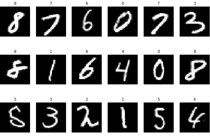
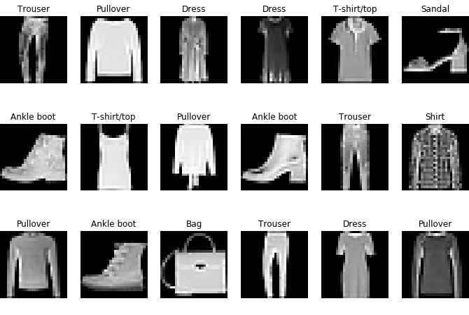
Sample Images

To get an impression of what the images look like, you can see some random samples below.

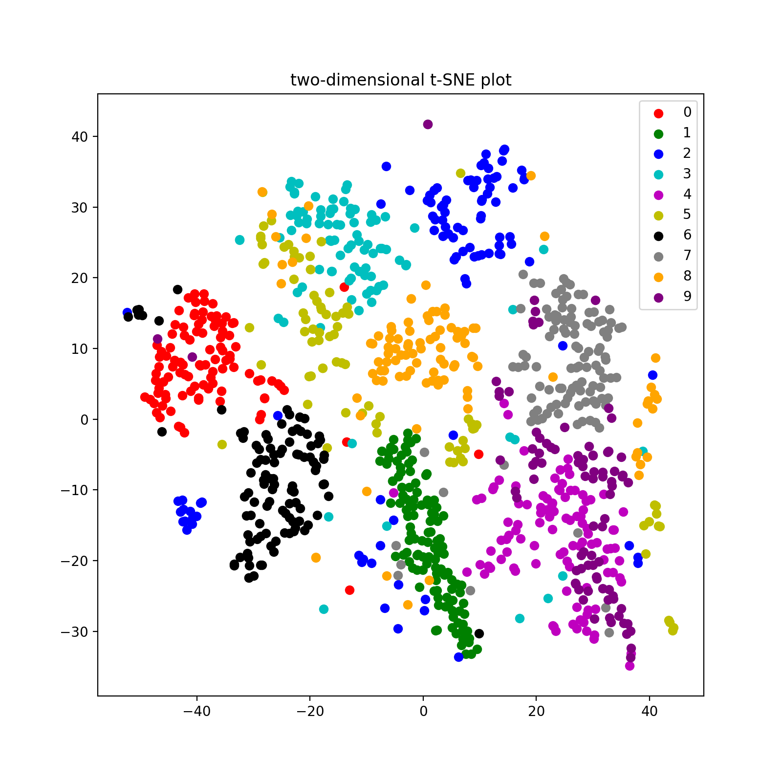
It is often useful to look at your data in as many ways as possible. We've already looked at the most obvious representation: images! Another way of looking at the data is as a collection of high-dimensional vectors (784 to be precise), where every number in the vector corresponds to the pixel intensity. Because it is not very practical to visualize high-dimensional vectors, several techniques exist that map these high-dimensional vectors to low-dimensional vectors such that I can show them in two or three dimensional space.

One of the most used dimensionality reduction techniques is t-SNE [3]. For more information and beautiful visualizations of t-SNE I can really recommend this website. It is outside the scope of this post to explain the exact workings of t-SNE. For now, the main gist is that the technique maps the high-dimensional vectors to low-dimensional vectors such that with a large probability the similar vectors in high dimensional space are also similar in low dimensional space. Similarly, the dissimilar vectors in high dimensional space have a low probability of being similar in low dimensional space.

Neural Networks

I could introduce you to a thousand and one interesting neural network architectures, but since the aim of this post is to give a simple introduction I will only focus on a single neural network. For this I choose a basic Convolutional Neural Network (CNN), a simple but yet powerful technique that was introduced already in 1998 [6]. Below you can see the (Pytorch) code that I used in the experiments.

class CONV(nn.Module):
    def __init__(self):
        super(CONV, self).__init__()
        self.conv1 = nn.Conv2d(1, 20, 5, 1)
        self.conv2 = nn.Conv2d(20, 50, 5, 1)
        self.fc1 = nn.Linear(4*4*50, 500)
        self.fc2 = nn.Linear(500, 10)

    def forward(self, x):
        x = F.relu(self.conv1(x))
        x = F.max_pool2d(x, 2, 2)
        x = F.relu(self.conv2(x))
        x = F.max_pool2d(x, 2, 2)
        x = x.view(-1, 4*4*50)
        x = F.relu(self.fc1(x))
        x = self.fc2(x)
        return x

Experiments

The networks are trained for 10 epochs, meaning that every image is presented 10 times to the network. After training the results are as follows:

• Train accuracy on MNIST: 99.6%
• Test accuracy on MNIST: 99.1%
• Train accuracy on Fashion-MNIST: 91.7%
• Test accuracy on Fashion-MNIST: 90.0%

As expected the accuracy on the MNIST dataset is higher than the accuracy on Fashion-MNIST (this was one of the main reasons to use Fashion-MNIST in the first place).

Besides showing the train accuracy I also show the test accuracy, this is a very important measure. The test accuracy is determined using images that are not presented to the network. If the train accuracy is significantly higher than the test accuracy, the network probably learned the images in the train set by hard. This could cause a low test accuracy since the network is no longer able to generalize to unseen data (this phenomenon is known as overfitting).

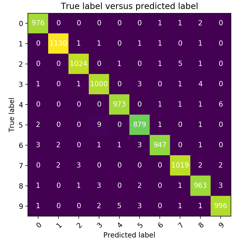
For the Fashion-MNIST dataset the confusion matrix is more interesting. You can directly see that the images that have the class shirt are difficult to predict for the network. Not only that, the network also wrongly predicts a lot of images to be of the class shirt. The first type of mistakes are known as false negatives (images of the class shirt are incorrectly predicted to not be of that class). The second type of mistakes are called false positives (the network incorrectly predicts images to be of the class shirt).

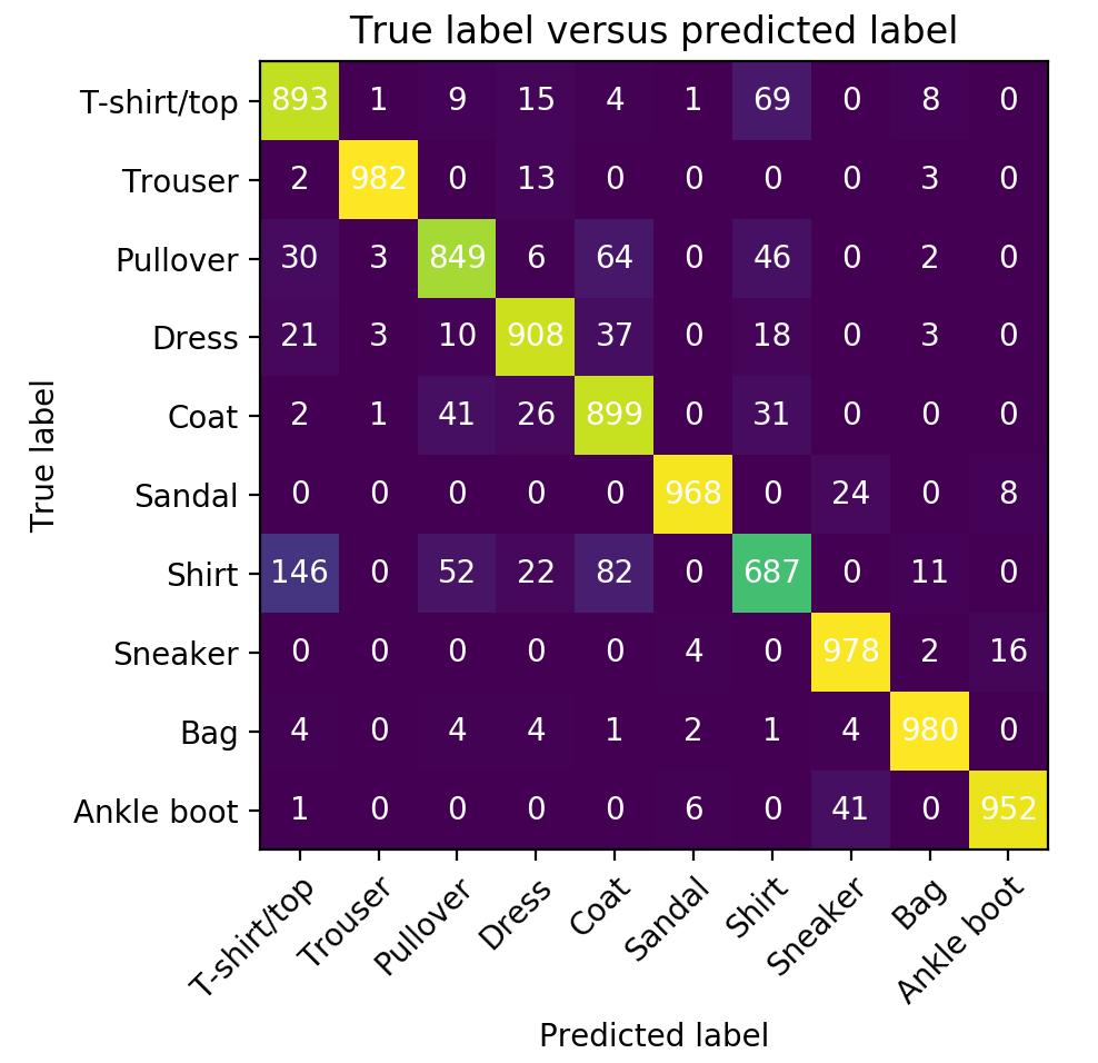
If you look more closely at what kind of mistakes the network makes, it is often the case that a misclassified image is predicted to be of a class that looks similar to humans (e.g. shirt vs coat or ankle boot vs sandal). This is not really a surprise since a CNN processes images in a similar way as humans do.

Transfer Learning

A large part of learning to classify images is learning what the images in the dataset actually consitute of. For both MNIST and Fashion-MNIST the network has to learn that the objects consist of primitives such as lines of varying angles, and edges. Since a lot of these primitives are present in both datasets, we can (hopefully) use the learned primitives of one dataset to classify images of the other dataset.

In order to test this I use the following procedure. First I train the network on both datasets for 10 epochs, after this I save the weights of the networks such that it is possible to restore them later on. Then, I load the MNIST dataset and restore the weights of the network that was trained on Fashion-MNIST. Similarly, I restore the weights of the network trained on MNIST, and use these to train on Fashion-MNIST.

In order to test transfer learning I use only 1000 images to train the network. If the network has indeed learned primitives that are transferable to another dataset, we expect that the accuracy is higher if we restore the weights compared to when we random initialize the weights. After training the network using only 1000 images for a single epoch, we find the following accuracies on the test set:

• Test accuracy on MNIST with transfer learning: 70.4%
• Test accuracy on MNIST without transfer learning: 14.5%
• Test accuracy on Fashion-MNIST with transfer learning: 52.0%
• Test accuracy on Fashion-MNIST without transfer learning: 16.3%

Clearly the algorithm performs better when we use the weights of a previously trained network, even if this network was trained on other data. Transfer learning can be very useful if you have little data to train on, but are in possession of a similar dataset. Furthermore, if you have already trained a network on a similar dataset, transfer learning might help you to speed up training.

Conclusion

In this blog post I showed you some basic machine learning techniques. The main goal was to introduce you to some concepts, rather than doing actual scientific experiments. I illustrated that even a simple network can achieve good results on two datasets. Furthermore, I showed that using transfer learning it is possible to get a relative high accuracy with very few images.

In future blog posts I will discuss a wild variety of topics. Some posts will be similar to this one, containing some introductory machine learning topics. In other posts I plan to go into more depth, and explain everything about a very specific algorithm. Please let me know if you have a request for a certain topic!

References

[1] LeCun, Yann. "The MNIST database of handwritten digits." http://yann.lecun.com/exdb/mnist/ (1998).

[2] Xiao, Han, Kashif Rasul, and Roland Vollgraf. "Fashion-mnist: a novel image dataset for benchmarking machine learning algorithms." arXiv preprint arXiv:1708.07747 (2017).

[3] Maaten, Laurens van der, and Geoffrey Hinton. "Visualizing data using t-SNE." Journal of machine learning research 9.Nov (2008): 2579-2605.

[4] Goodfellow, Ian, et al. "Generative adversarial nets." Advances in neural information processing systems. (2014).

[5] Sabour, Sara, Nicholas Frosst, and Geoffrey E. Hinton. "Dynamic routing between capsules." Advances in Neural Information Processing Systems. (2017).

[6] LeCun, Yann, et al. "Gradient-based learning applied to document recognition." Proceedings of the IEEE 86.11 (1998): 2278-2324.