What bird is that? Bird detection using machine learning

This is a series of posts on how we can build a bird classification system using machine learning. In my previous post I started by exploring the characteristics of sound (data) and we ended that post by generating mel spectrograms for two randomly selected bird songs. In this post we will actually start classifying recordings. More specifically, we will train a model to predict whether a short recording contains a bird sound. Let's dive in!

Our end goal is of course to build a system that can classify birds based on the sounds they make. However, this leaves us with a problem if there are no birds present in a recording. One solution could be to make a fake bird species called 'no-bird', where we map all empty recordings to. This way, a model can learn to predict this class whenever it doesn't detect any bird in a recording. However, in general there will be way more recordings without birds than recordings with a specific kind of bird, which would most likely harm the performance of such a classification model. Therefore, we will train two separate models:

1. A model that only predicts whether there is a bird present in a recording or not
2. A model that only comes into play when the first model detects a bird and will try to predict which kind of bird we are hearing

In this post we will have a look at the first model. We will collect a dataset of recordings, extract features from these recordings, build a convolutional neural network (CNN) and train it to predict whether a bird is present in a given recording.

The Dataset

For this binary prediction model, we need a dataset that represents the natural habitat of birds. Luckily, there exists a challenge that focuses exactly on the problem we are dealing with. In the DCASE - Bird audio detection challenge, the task is to build a system that, given a short audio recording, returns a binary decision for the presence/absence of bird sound.

The data used in this challenge comes from five different datasets. Some of these datasets are crowdsourced, while others are constructed from remote-monitoring projects. The latter have the advantage of generally being more diverse, as crowdsourced datasets are often recordings made during daytime in good weather conditions. The three datasets that are used as training data together contain over 35 thousand recordings, so this should be sufficient to train our model.

After looking at the results of this challenge, we found that the model by the UKYSpeechLab was the highest scoring open-source submission. After reading their paper, we found that the difference in performance between their baseline model and best performing model was relatively small. Therefore, we decided to focus on their baseline model. This model is actually an adapted version of the winner of the 2017 DCASE challenge, called Bulbul.

Convolutional Neural Networks

This neural network consists of four 2 dimensional convolutional layers followed by three fully connected layers. Since feeding the raw audio recordings to a neural network is not very practical, the log mel-spectrogram is used in many of the submissions for this challenge. In case you are wondering what this is, have a look at my previous post in this series.

A convolutional neural network is a neural network that contains at least one convolutional layer. These networks are often used to classify images. A convolutional layer convolves, an operation similar to multiplication, the input image with filters to detect certain features in the input image.

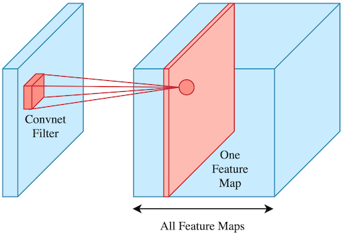
Convolution operation with left the input image (blue) and the filter. On the right you see the resulting feature map (red) after convolving the image with the filter. This is repeated for all filters, which gives you all the feature maps. (Source)

If we look at what a CNN actually learns, we can often observe some very interesting patterns. Generally speaking, the first convolutional layer looks for more general features such as edges and colours. As we progress through the network the features become more specific.

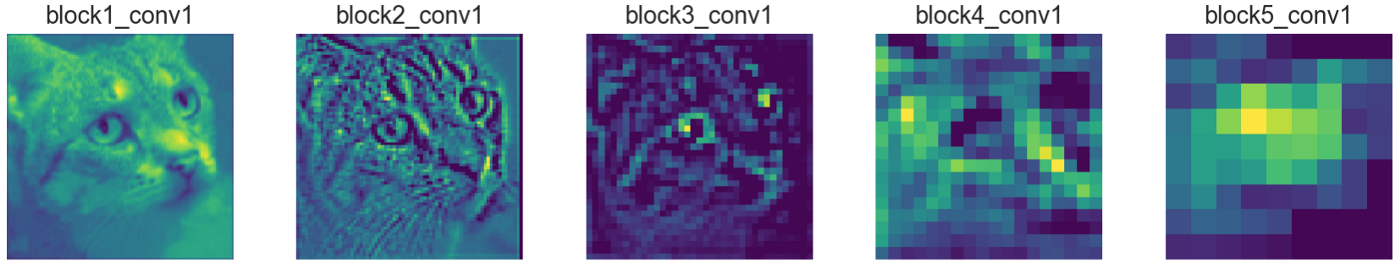
Feature maps of several convolutional layers in a network that learns to recognise cats. (Source)

CNNs are often used for image data, so why are we using it here? Well as discussed in the previous post, both image and audio data are stored as numbers on our computer. In fact, we can visualise the log mel-spectrogram as an image as can be seen in the image below. In our case the log mel-spectrogram has the following dimensions (700,80,1). You think of it as a black and white image (only 1 channel) that is 700 by 80 pixels.

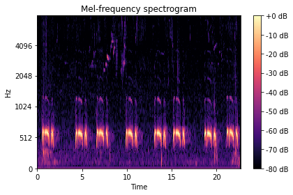
Mel-spectrogram example

Training Process and Results

The training process goes as follows. We randomly split the 35 thousand recordings into two sets: a training set and a test set. The first one is used during training, while the latter is only used after the model has finished training. Normally we would also use a validation set, which is a small set of data we can use while training to see how the model performs on data is hasn't trained on. However, since we are using a model that has proven to work for this task, we decided to use more data for training and not use a validation set.

So during training we feed the extracted log mel-spectrograms from the training set, where one entire run over the training data is called an epoch. We repeat this process 50 times. So after 50 epochs, we save the model and use it to predict the samples in our test set to see how well our model is able to handle these unseen (or heard) recordings.

So how did we do? Well first we should note that also the experts that annotated these 35 thousand samples didn't always agree. The average agreement between annotators on these datasets is 96.7%. So in a perfect world we would score an accuracy of around 97% on the unseen testing data. Although we didn't really get that far, we managed to obtain an accuracy of 92%.

Confusion matrix for the test set

If we want to look at the mistakes our model makes, the confusion matrix is a handy visualisation. It shows the kind of mistakes the model makes, so whether it often predicts birds when there are none (false positives) or whether it misses birds in recordings that contain birds (false negatives). We can see that in 52 cases it misses a bird while there is one present and in 96 cases it predicts that there is a bird present while there is no bird present. Luckily, in the remaining 1628 cases the model is spot on!

So now that we have a neural network that, given a log mel-spectrogram of a recording, can tell us whether there is a bird present in the recording we can turn to the next challenge. Whenever our newly trained model detects a bird, we need to be able to classify it. We will build this model in the next post!