What bird is that? Bird sound classification using machine learning

This is a series of posts on how we can build a bird classification system using machine learning. In my previous post I showed how you can build a classifier that distinguishes between bird sounds and non bird sounds. In this post we will build a classifier that comes into play after our previous model detects a bird sound. We will build a model that predicts the type of bird that has been detected!

At first I was afraid that obtaining a dataset would be cumbersome. However, then I came across xeno-canto. Xeno-canto is a website where people from all over the world share sounds of wild birds. There are nearly half a million recordings of over 10 thousand species in their database. They even have an API, which we can use to download the data we are interested in.

Using this very nice series on bird classification, we were able to obtain a list of recordings from birds and were able to write a python script with which we downloaded over 150 thousand bird recordings made in Europe. So what do we have now? Well, a folder with 150 thousand audo files and a csv file with for every file some information on the location of the recording and the bird that is present in the recording.

Dataset Analysis

Next, we need to somehow convert these 150 thousand audio files and csv file to something we can work with. Let's first have a look at some characteristics of the data:

• We have recordings from 50 different countries and 656 different species
• The number of species using the English name is even higher with 724
• Most recordings are from the United Kingdom (almost 30 thousand)
• The class imbalance is quite severe, with over 5000 recordings from the Great Tit and only 1 from over 50 different species

Since the number of species is extremely large and for many species we have only 1 or 2 recordings, I decided to use the genus of the bird as target. This means we will not predict the actual species nor the family of the bird, but something in between. For example, the Great spotted woodpecker is part of the Dendrocopos genus which consists of woodpeckers from Asia, Europe and Northern Africa. The Dendrocopos genus is part of the Picidae family, which contains all woodpeckers. More information on genus, can be found here.

In total there are 353 different genera in our dataset. The most occurring genus is Turdus, to which the common black bird belongs. Since we want a diverse set of recordings for every class, we decided to remove all genera for which we have less than 1500 recordings. This leaves us, after removing irrelevant and non-complete recordings, with 80 thousand recordings. From these 80 thousand recordings we randomly selected 15 thousand (while preserving a balanced dataset) to use for this experiment.

Feature Extraction

Now that we have our final list of bird recordings, we can turn to feature extraction. Just as before, we will not be feeding the raw audio data to our model. Instead we will crop a window from every recording and generate a log mel spectrogram. I hope you still remember what this is, if not please have a look at the first post in this series. We will be using the exact same script as before, as to make sure we can use the same input in both the bird detection and bird classification model.

Model Architecture

So the task for the model will be to predict the genus of the bird that is present in the log mel spectrogram. But what model will we be using? Well, I decided to compare two models:

1. The first model is the same model as we have used in the previous post called Bulbul. This neural network consists of four 2 dimensional convolutional layers followed by three fully connected layers.
2. The second model we will use is called Resnet introduced in 2015 by He et al. This is a deep Convolutional Neural Network (CNN) that uses residual connections.

So what is so special about Resnet? Well, with the increase in computing power we were able to make deeper networks. This increase in the number of layers has caused networks to become more powerful. This can be clearly seen in the image below where we show an example of a Resnet. The network has 34 (!) layers.

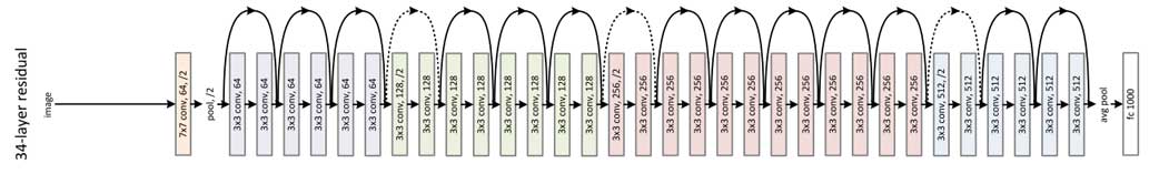
Resnet architecture (source)

However, more layers can also cause the loss of critical information. In the second image below we see the normal connections between the layers I-2, I-1, and I. If there is some information present in the features after applying layer I-2 that is relevant for layer I, but is lost due to the application of layer I-1, this information is lost forever. That is why a skip connection is introduced, which directly connects layers I-2 and I. By adding several of these skip connections in the network, we saw a tremendous increase in the performance of large models in 2015.

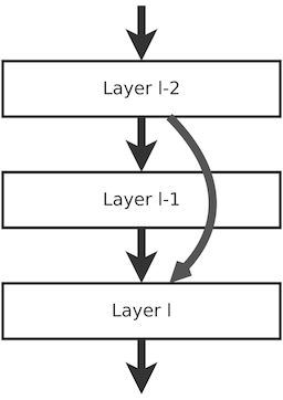
An example of a residual connection (source)

In more technical terms, these connections can help solve or at least alleviate the vanishing gradient problem. Neural nets learn through back propagating gradients. These gradients contain information on how to adapt the weights to improve performance. These gradients are found by calculating the partial derivative of the loss function with respect to the weights of the network. As networks become deeper these gradients sometimes become extremely small, especially for layers in the first part of the network. By adding skip connections, more information from the shallow parts of the network flows to the deeper parts, thus alleviating the vanishing gradient problem.

Results and Future Work

So how did we do? Well, on the unseen test set we were able to obtain an accuracy of:

• 70% using Bulbul
• 80% using Resnet

That is quite a bit lower than our previous model scored on the bird detection task (92%), which makes sense given that in that task there are only two classes, while here we have 22 classes. Furthermore, I did not spend much time on hyperparameter tuning, used only a small portion of the available data and tested relatively simple models. I suspect there is still some room for improvement.

Let's go back to our first post in this series. I noticed that I often worked with either text or images and wanted to learn more about applying machine learning on audio. We learned:

• How audio data is represented
• Features we can extract from audio files
• How CNNs work
• What kind of models perform well in bird detection challenges
• Scraping the internet for audio recordings from all over the world
• What skip connections do

We now have a model that can distinguish between bird sounds and non bird sounds with 92% accuracy and a model that can predict the genus of a bird given with 80% accuracy. I think we have two things left to do:

1. Investigate how we can improve the performance of our models by experimenting with different network architectures and hyperparameters
2. Deploying our models in the wild

The next post in this series will look at improving our bird detection and classification models. We will dive in the different kind of layers we can add to our networks and how we can make changes to the architecture that increase performance. Moreover, we will have a look at the different parameters that come into play and how we can tune these to increase the performance of our models. After that, we will try to actually deploy our models. And with that I do not mean deploying to the cloud...